As a Customer Success Engineer at Looker, in addition to guiding customers on their data architecture, I also regularly build out technical solutions for our internal customer success functions. The one I’m going to be sharing today is our predictive renewal score, and the technologies I’ll be demonstrating are Looker and BigQuery’s Machine Learning service, which combine to make this end-to-end solution super fast to build out, enhance, and maintain.
So, what is this predictive renewal score? A score from 0 to 100% that estimates the likelihood that a given customer will renew. In practice, it actually has a few distinct functions within our organization -
- Summarizing score - When a Customer Success Manager or Account Executive wants to get a feel for a specific account, this is a composite score that can help them get a quick first sense for where the customer is overall, without having to individually consider and integrate dozens of aspects of the customer’s profile. To help with this, I also color code the score into three tiers - red/yellow/green.
- Prioritization feature - When a Customer Success Manager wants to proactively allocate their time within a pool of accounts, they can use this score in a first pass over a list to help in prioritizing.
- Forecasting input - Since the score represents a probability of renewing, we can use it for forecasting. We simply multiply it by the account’s Annual Contract Value and sum up these products to get the total expected dollars renewing across a set of accounts. We can slice and dice this by account owners, account segments, regions, etc.
The end result is - the score helps us understand and reduce customer churn. Hopefully, you see some similar opportunities for a similar score in your own organization. Let’s dive in to how to build it!
LookML for Structure
We’ll be using LookML to keep everything organized. In my case, this solution exists inside of a much larger LookML project, and is relatively stand-alone, so I’m going to be putting all of these into one file to keep the larger project tidy. In addition, I’ve prefixed all the views, to make them play more nicely within the larger project namespace. Finally, I’m using primary key naming conventions from my LookML Style Guide to help make the join logic more transparent and reliable.
What Do We Want?!
So, let’s start by defining what we’ll be predicting. In our case, we’re using Saleforce opportunities, and specifically ones with type “Renewal”. A simple view will help us organize this dataset of interest. We’ll start FROM salesforce.opportunity, apply a WHERE filter on type='Renewal' and within a certain timeframe, and convert the stage_name to a binary outcome.
See the code - Objectives
view: prs_objectives {
derived_table: {
sql:
SELECT
opp.id as pk1_opportunity_id,
---
start_date as date,
opp.account_id as entity_id, --See note #1
CASE opp.stage_name
WHEN 'Closed Won' THEN 1
WHEN 'Closed Lost' THEN 0
ELSE NULL
END as result
FROM `salesforce.opportunity` as opp
CROSS JOIN UNNEST([ --See note #2
COALESCE(opp.start_date__c, opp.close_date)
]) as start_date
WHERE opp.type='Renewal'
AND start_date >= DATE_ADD(CURRENT_DATE(), INTERVAL 0-(2*365) DAY)
-- Taking renewals up to two years in the past
AND DATE_DIFF(start_date, CURRENT_DATE(), MONTH)<>0
-- ^ Current month neither needs prediction, nor is settled enough to use for training
;;
}
dimension: pk1_opportunity_id {hidden:yes}
dimension: date {hidden:yes}
dimension: entity_id {hidden:yes}
dimension: result {hidden:yes description: "The objective of the prediction, either a 0 or 1."}
}
**Notes for the above query**
- I've chosen to alias the account_id as "entity_id" to describe the abstract function for which we are using the account ID here. Namely, multiple opportunities under an account will care about the history of events for the account/entity as a whole, even if there was another opportunity recently. This abstraction should help apply this pattern to other datasets.
- `CROSS JOIN UNNEST ([expression]) as alias` is a bit confusing to read at first. Technically, it's joining for each row on the left of the join a single-row, single-column "table" defined by the expression. In practice, it's essentially creating an alias or projection which can be reused without writing out the whole expression. (This is similar to a LATERAL JOIN in other dialects)
If your dataset doesn’t have explicit opportunities already defined, you can easily create your own stand-in opportunities by taking your customers and joining them against a year, month or date table.
When Do We Want It?!
With the scope of our problem defined, I’ll need to take a brief aside into when predictions are made and how this time element interacts with the prediction itself.
Since our organization operates on yearly contracts, the opportunities that we want to predict are relatively sparse. We’ll definitely want to be updating our predictions multiple times over the course of a year for any given opportunity, rather than having one specific prediction per opportunity.
In our case, many of our business operations are aligned to months, so we’ll align with that too to avoid fatiguing or distracting users with super frequent updates. That means that each month, we’ll be generating a new prediction for every future opportunity, whether it is next month, or 12+ months away. In addition, because some patterns of usage are leading indicators of success and some are more lagging, we’ll include how far out the renewal is as a feature in the dataset, so our model can theoretically weight features differently if they are more important earlier or later in a renewal cycle.[1]
This has implications for my training data set - I want to make it comparable to the data I will eventually use for prediction. Specifically, since I will be predicting renewals that happen both next month all the way to 12 months from now, I’d like the training data to also have datapoints representative of those situations.
In our LookML/SQL, I call this concept lead_periods. Whenever a renewal is in the training dataset, I cross join it with a 12-row number table, and calculate the date that many months before the renewal. For example -
| Renewal ID |
Renewal Date |
Result |
Lead Periods |
Lead Date |
| A |
6/1/2018 |
1 |
1 |
5/1/2018 |
| A |
6/1/2018 |
1 |
2 |
4/1/2018 |
| … |
… |
… |
… |
… |
| A |
6/1/2018 |
1 |
12 |
6/1/2017 |
| B |
9/1/2018 |
0 |
1 |
8/1/2018 |
| … |
… |
… |
… |
… |
From here, I can easily take one or more date-windowed datasets and join them onto those “lead dates”, even if there is overlap between the windows and multiple lead dates. For example, if one of the features in the dataset were “how many users used the service in the trailing 8 weeks?”, then most days in our raw usage data would need to affect multiple datapoints in the “lead dates” result. By having the trailing happen in a window function, we can easily handle these cases.
See the code - Dataset with Lead Periods
view: prs_dataset {
derived_table: {
persist_for: "2 hours"
sql:
SELECT
-- Primary Keys
objectives.pk1_opportunity_id as pk2_opportunity_id,
lead_periods.n as pk2_lead_periods,
---
-- `subset` will be used later to split this dataset
CASE
WHEN DATE_DIFF(CURRENT_DATE(),objectives.date,MONTH)<0
THEN "prediction"
WHEN DATE_DIFF(CURRENT_DATE(),objectives.date,MONTH)>1 AND objectives.result IS NOT NULL
THEN "training"
WHEN DATE_DIFF(CURRENT_DATE(),objectives.date,MONTH)=1 AND objectives.result IS NOT NULL
THEN "holdout"
ELSE "ignore" -- CURRENT MONTH OR PAST NULL RESULT
END
AS subset,
CASE WHEN DATE_DIFF(CURRENT_DATE(),objectives.date,MONTH)<0
THEN NULL
ELSE objectives.result
END as result,
-- Any number of additional features
activity.usage_minutes_w1to4,
ROUND(activity.usage_minutes_w1to4 / NULLIF(licensing.users,0),2) as minutes_per_user,
ROUND(activity.minutes_w1to4 / NULLIF(activity.minutes_w25to28,0),2) as minutes_trend,
--etc...
-- The first two tables set up the right rows in the result set
FROM ${prs_objectives.SQL_TABLE_NAME} AS objectives
INNER JOIN ${prs_numbers_1_to_12.SQL_TABLE_NAME} as lead_periods
ON CASE
WHEN objectives.result IS NOT NULL
THEN TRUE
ELSE lead_periods.n = LEAST(12, DATE_DIFF(objectives.date,CURRENT_DATE(),MONTH))
END
-- This maps lead_periods to a specific date for joining further tables
LEFT JOIN ${prs_dates.SQL_TABLE_NAME} as prediction_date
ON prediction_date.pk1_date = CASE
WHEN objectives.result IS NOT NULL
THEN DATE_TRUNC(DATE_ADD(
objectives.date,
INTERVAL (0 - lead_periods.n) MONTH
), MONTH)
ELSE DATE_TRUNC(CURRENT_DATE(), MONTH)
END
-- Continue with any number of 1:1 or m:1 joins
LEFT JOIN ${prs_activity.SQL_TABLE_NAME} as activity
ON activity.pk2_entity_id = objectives.entity_id
AND activity.pk2_date = prediction_date.pk1_date
LEFT JOIN ${prs_licensing.SQL_TABLE_NAME} as licensing
ON licensing.pk2_entity_id = objectives.entity_id
AND licensing.pk2_date = prediction_date.pk1_date
LEFT JOIN ${account.SQL_TABLE_NAME} as account
ON account.id = objectives.entity_id
;;
}
dimension: pk2_opportunity_id {hidden:yes}
dimension: pk2_lead_periods {hidden:yes}
dimension: subset {}
dimension: result {}
extends: [psr_features]
}
Enter BigQuery Machine Learning
Before I rebuilt this solution on BQML, going from dataset to predictions was a painful manual process. Once the model was trained, I would schedule the dataset to myself on a monthly basis, upload it into a third-party ML service, click a bunch of buttons, download a CSV, reformat my CSV to NDJSON, and ETL it back into our datawarehouse. And updating the model? If I got around to that in 6 months’ time, that would already be a miracle.
Now? New predictions happen automatically, retraining happens automatically, and running a new model is just a page refresh.
And not only does automatic mean less strife for me, it means I can now do more - like create multiple predictive scores based on different feature sets to help business users understand different facets of a customer’s health. Maybe a customer is “yellow” overall, but “green” in terms of communication & contact, but “yellow” in terms of product usage & adoption - now that’s actionable.
But, I digress - Let’s see the (surprisingly short) setup in LookML!
See the code - Model & Prediction
view: prs_model {
derived_table: {
datagroup_trigger: first_of_the_month
sql_create:
CREATE OR REPLACE MODEL ${SQL_TABLE_NAME}
OPTIONS (
model_type='logistic_reg',
input_label_cols=['result'],
l1_reg=0.025,
l2_reg=0.025
)
AS (
SELECT * EXCEPT (pk2_opportunity_id)
FROM ${prs_dataset.SQL_TABLE_NAME}
WHERE subset = 'training'
);;
}
}
view: prs_prediction {
derived_table: {
datagroup_trigger: first_of_the_month
sql:
SELECT * FROM ML.PREDICT(
MODEL ${prs_model.SQL_TABLE_NAME},
( SELECT * EXCEPT (result)
FROM ${prs_dataset.SQL_TABLE_NAME}
WHERE subset = 'prediction'
)
);;
}
dimension: pk1_opportunity_id {hidden:yes sql:${TABLE}.pk2_opportunity_id;;}
extends: [prs_features]
dimension: predicted_result {type: number}
dimension: renewal_prob {type: number sql:(SELECT prob FROM UNNEST(${TABLE}.predicted_result_probs) WHERE label=1);; value_format_name: percent_2}
}
Inspection
In addition to simply training and running the model, let’s add a bit of instrumentation so we can summarize what happened during our training and the quality of our model. We’ll use both some of the static evaluation functions that BigQuery provides, but also comparisons between the predictions and actuals for our holdout set (last month’s renewals).
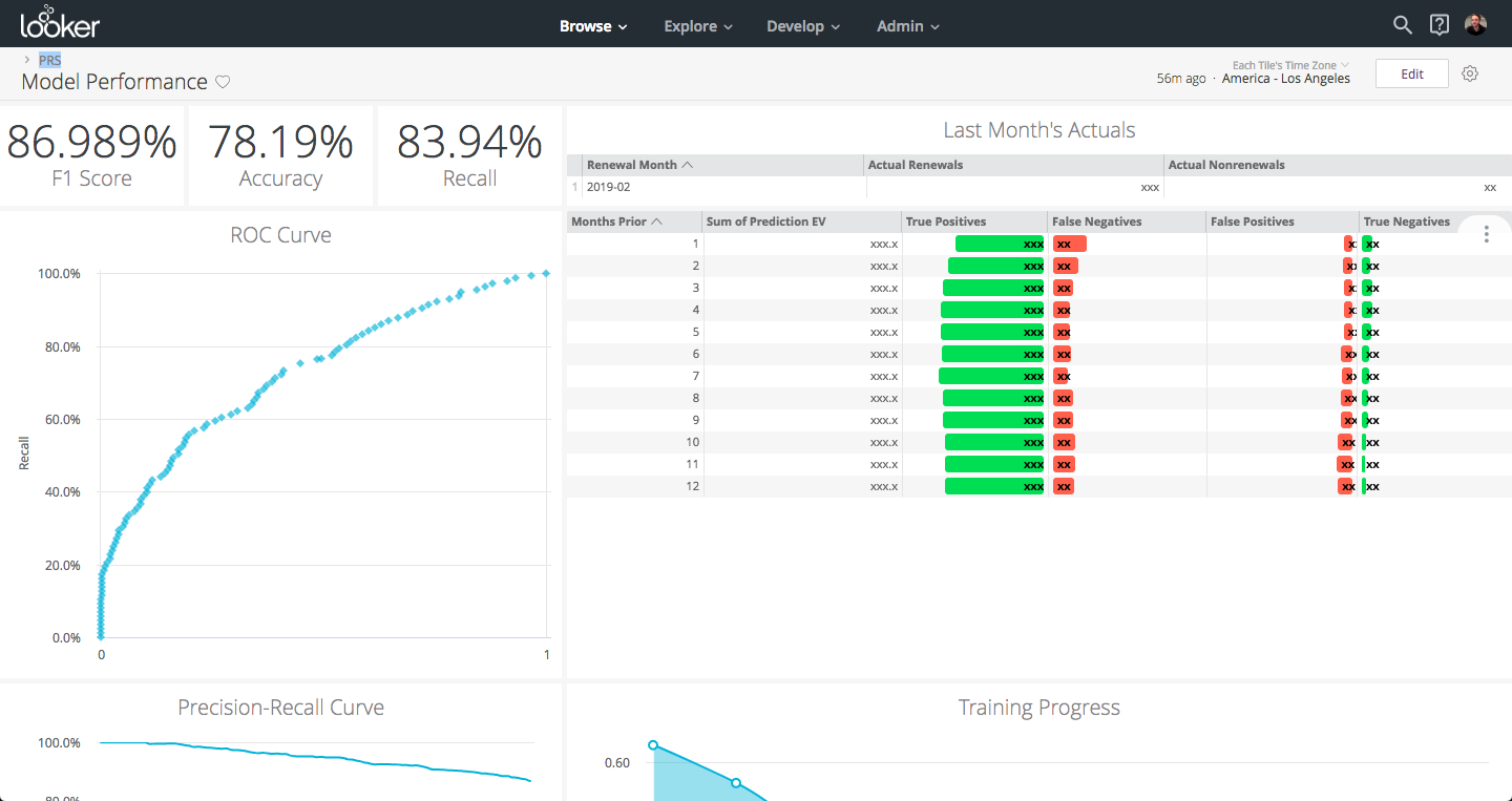
As an added bonus, the model inspection dashboard in dev mode makes a great place to trigger re-training of our model whenever we update the feature set in our SQL. Since Looker already maintains separate SQL table names for changes we make in dev mode, we can safely test out features in our dev mode without affecting the model and predictions in production.
See the code - LookML
explore: prs_holdout {extends: [prs_joins]}
explore: prs_evaluation {hidden:yes}
explore: prs_roc {hidden:yes}
explore: prs_training_info {hidden:yes}
# Some logic borrowed from https://github.com/llooker/bqml_ga_demo/blob/master/predictions.view.lkml
view: prs_evaluation {
derived_table: {
sql: SELECT * FROM ml.EVALUATE(
MODEL ${prs_model.SQL_TABLE_NAME},
TABLE ${prs_holdout.SQL_TABLE_NAME}
);;
}
dimension: recall {type: number value_format_name:percent_2}
dimension: accuracy {type: number value_format_name:percent_2}
dimension: f1_score {type: number value_format_name:percent_2}
dimension: log_loss {type: number}
dimension: roc_auc {type: number}
}
view: prs_roc {
derived_table: {
sql: SELECT * FROM ml.ROC_CURVE(
MODEL ${prs_model.SQL_TABLE_NAME},
TABLE ${prs_holdout.SQL_TABLE_NAME}
);;
}
dimension: threshold {type: number}
dimension: recall {type: number value_format_name: percent_1}
dimension: false_positive_rate {type: number value_format_name: percent_1}
dimension: true_positives {type: number }
dimension: false_positives {type: number}
dimension: true_negatives {type: number}
dimension: false_negatives {type: number }
dimension: precision {type: number value_format_name: percent_1
sql: ${true_positives} / NULLIF((${true_positives} + ${false_positives}),0);;
}
dimension: threshold_accuracy {type: number value_format_name: percent_1
sql: 1.0*(${true_positives} + ${true_negatives}) / NULLIF((${true_positives} + ${true_negatives} + ${false_positives} + ${false_negatives}),0);;
}
dimension: threshold_f1 {type: number value_format_name: percent_1
sql: 2.0*${recall}*${precision} / NULLIF((${recall}+${precision}),0);;
}
measure: total_false_positives {type: sum sql: ${false_positives} ;;}
measure: total_true_positives {type: sum sql: ${true_positives} ;;}
}
view: prs_training_info {
derived_table: {
sql: SELECT * FROM ml.TRAINING_INFO(MODEL ${prs_model.SQL_TABLE_NAME});;
}
dimension: training_run {type: number}
dimension: iteration {type: number}
dimension: eval_loss {type: number}
dimension: duration_ms {label:"Duration (ms)" type: number}
dimension: learning_rate {type: number}
measure: total_iterations {type: count}
measure: loss {type: sum value_format_name: decimal_2 sql: ${TABLE}.loss;; }
measure: total_training_time {type: sum value_format_name: decimal_1
label:"Total Training Time (sec)"
sql: ${duration_ms}/1000 ;;
}
measure: average_iteration_time {
type: average
label:"Average Iteration Time (sec)"
sql: ${duration_ms}/1000 ;;
value_format_name: decimal_1
}
}
view: prs_holdout{
derived_table: {
datagroup_trigger: first_of_the_month
sql:
SELECT * FROM ML.PREDICT(
MODEL ${prs_model.SQL_TABLE_NAME},
( SELECT *
FROM ${prs_dataset.SQL_TABLE_NAME}
WHERE subset = 'holdout'
)
)
;;
}
dimension: pk2_opportunity_id {hidden:yes}
dimension: pk2_date {hidden:yes}
extends: [prs_features]
dimension: result {type: number}
dimension: predicted_result {type: number}
dimension: renewal_prob {type: number sql:(SELECT prob FROM UNNEST(${TABLE}.predicted_result_probs) WHERE label=1);; value_format_name: percent_2}
measure: count {type:count drill_fields: [account.name, renewal_prob, predicted_result, result]}
measure: predicted_renewals {type:sum sql:${predicted_result};;}
measure: predicted_nonrenewals {type:sum sql:1-${predicted_result};;}
measure: ev_renewals {type:sum sql:${renewal_prob};; value_format_name:decimal_1}
measure: actual_renewals {type:sum sql:${result};;}
measure: actual_nonrenewals {type:sum sql:1-${result};;}
measure: false_positives {
type:count
filters: {field: predicted_result value: "1"}
filters: {field: result value:"0"}
drill_fields: [account.name, renewal_prob, predicted_result, result]
html:
;;
}
measure: true_positives {
type:count
filters: {field: predicted_result value: "1"}
filters: {field: result value:"1"}
drill_fields: [account.name, renewal_prob, predicted_result, result]
html:
;;
}
measure: false_negatives {
type:count
filters: {field: predicted_result value: "0"}
filters: {field: result value:"1"}
drill_fields: [account.name, renewal_prob, predicted_result, result]
html:
;;
}
measure: true_negatives {
type:count
filters: {field: predicted_result value: "0"}
filters: {field: result value:"0"}
drill_fields: [account.name, renewal_prob, predicted_result, result]
html:
;;
}
measure: percent_fp {
hidden: yes type: number value_format_name: percent_1
sql: ${false_positives}/${count} ;;
}
measure: percent_fn {
hidden: yes type: number value_format_name: percent_1
sql: ${false_negatives}/${count} ;;
}
measure: percent_tp {
hidden: yes type: number value_format_name: percent_1
sql: ${true_positives}/${count} ;;
}
measure: percent_tn {
hidden: yes type: number value_format_name: percent_1
sql: ${true_negatives}/${count} ;;
}
}
See the code - Dashboard
- dashboard: model_performance
title: Model Performance
layout: newspaper
elements:
- title: Training Progress
name: Training Progress
model: bq_salesforce
explore: prs_training_info
type: looker_area
fields: [prs_training_info.loss, prs_training_info.iteration]
sorts: [prs_training_info.iteration]
limit: 500
query_timezone: America/New_York
stacking: ''
show_value_labels: false
label_density: 25
legend_position: center
x_axis_gridlines: false
y_axis_gridlines: true
show_view_names: false
point_style: circle_outline
limit_displayed_rows: false
y_axis_combined: true
show_y_axis_labels: true
show_y_axis_ticks: true
y_axis_tick_density: default
y_axis_tick_density_custom: 5
show_x_axis_label: true
show_x_axis_ticks: true
x_axis_scale: auto
y_axis_scale_mode: linear
x_axis_reversed: false
y_axis_reversed: false
show_null_points: true
interpolation: monotone
show_totals_labels: false
show_silhouette: false
totals_color: "#808080"
series_types: {}
listen: {}
row: 11
col: 9
width: 15
height: 8
- title: Accuracy
name: Accuracy
model: bq_salesforce
explore: prs_evaluation
type: single_value
fields: [prs_evaluation.accuracy]
sorts: [prs_evaluation.accuracy]
limit: 500
query_timezone: America/New_York
custom_color_enabled: false
custom_color: forestgreen
show_single_value_title: true
show_comparison: false
comparison_type: value
comparison_reverse_colors: false
show_comparison_label: true
listen: {}
row: 0
col: 3
width: 3
height: 2
- title: Recall
name: Recall
model: bq_salesforce
explore: prs_evaluation
type: single_value
fields: [prs_evaluation.recall]
sorts: [prs_evaluation.recall]
limit: 500
query_timezone: America/New_York
custom_color_enabled: false
custom_color: forestgreen
show_single_value_title: true
show_comparison: false
comparison_type: value
comparison_reverse_colors: false
show_comparison_label: true
listen: {}
row: 0
col: 6
width: 3
height: 2
- title: F1 Score
name: F1 Score
model: bq_salesforce
explore: prs_evaluation
type: single_value
fields: [prs_evaluation.f1_score]
sorts: [prs_evaluation.f1_score]
limit: 500
query_timezone: America/New_York
custom_color_enabled: false
custom_color: forestgreen
show_single_value_title: true
show_comparison: false
comparison_type: value
comparison_reverse_colors: false
show_comparison_label: true
listen: {}
row: 0
col: 0
width: 3
height: 2
- title: ROC Curve
name: ROC Curve
model: bq_salesforce
explore: prs_roc
type: looker_scatter
fields: [prs_roc.recall, prs_roc.false_positive_rate]
limit: 500
column_limit: 50
stacking: ''
show_value_labels: false
label_density: 25
legend_position: center
hide_legend: true
x_axis_gridlines: true
y_axis_gridlines: true
show_view_names: false
point_style: circle
series_colors:
_: "#d5d7db"
series_types: {}
series_point_styles:
prs_roc.recall: diamond
limit_displayed_rows: false
y_axes: [{label: '', orientation: left, series: [{id: prs_roc.total_true_positives,
name: Total True Positives, axisId: prs_roc.total_true_positives,
__FILE: bq_salesforce/oo.prs.dashboard.lookml, __LINE_NUM: 318},
{id: _, name: "-", axisId: _, __FILE: bq_salesforce/oo.prs.dashboard.lookml,
__LINE_NUM: 321}], showLabels: false, showValues: true, unpinAxis: false,
tickDensity: default, tickDensityCustom: 5, type: linear, __FILE: bq_salesforce/oo.prs.dashboard.lookml,
__LINE_NUM: 315}]
y_axis_combined: true
show_y_axis_labels: true
show_y_axis_ticks: true
y_axis_tick_density: default
y_axis_tick_density_custom: 5
show_x_axis_label: false
show_x_axis_ticks: true
x_axis_scale: linear
y_axis_scale_mode: linear
x_axis_reversed: false
y_axis_reversed: false
plot_size_by_field: false
reference_lines: []
trend_lines: []
show_null_points: true
interpolation: monotone
ordering: none
show_null_labels: false
show_totals_labels: false
show_silhouette: false
totals_color: "#808080"
hidden_fields: []
listen: {}
row: 2
col: 0
width: 9
height: 9
- title: Precision-Recall Curve
name: Precision-Recall Curve
model: bq_salesforce
explore: prs_roc
type: looker_line
fields: [prs_roc.precision, prs_roc.recall]
sorts: [prs_roc.precision]
limit: 500
query_timezone: America/New_York
stacking: ''
show_value_labels: false
label_density: 25
legend_position: center
x_axis_gridlines: false
y_axis_gridlines: true
show_view_names: false
point_style: none
limit_displayed_rows: false
y_axis_combined: true
show_y_axis_labels: true
show_y_axis_ticks: true
y_axis_tick_density: default
y_axis_tick_density_custom: 5
show_x_axis_label: true
show_x_axis_ticks: true
x_axis_scale: auto
y_axis_scale_mode: linear
x_axis_reversed: false
y_axis_reversed: false
show_null_points: true
interpolation: monotone
series_types: {}
y_axes: [{label: '', orientation: left, series: [{id: prs_roc.precision,
name: Precision, axisId: prs_roc.precision, __FILE: bq_salesforce/oo.prs.dashboard.lookml,
__LINE_NUM: 462}], showLabels: true, showValues: true, unpinAxis: false,
tickDensity: default, tickDensityCustom: 5, type: linear, __FILE: bq_salesforce/oo.prs.dashboard.lookml,
__LINE_NUM: 459}]
x_axis_datetime_label: ''
hide_legend: false
listen: {}
row: 11
col: 0
width: 9
height: 8
- title: vs Simulated Historical Predictions
name: vs Simulated Historical Predictions
model: bq_salesforce
explore: prs_holdout
type: table
fields: [prs_holdout.lead_periods, prs_holdout.ev_renewals, prs_holdout.true_positives,
prs_holdout.false_negatives, prs_holdout.false_positives, prs_holdout.true_negatives]
sorts: [prs_holdout.lead_periods]
limit: 500
query_timezone: America/Los_Angeles
show_view_names: false
show_row_numbers: false
truncate_column_names: false
subtotals_at_bottom: false
hide_totals: false
hide_row_totals: false
series_labels:
prs_holdout.lead_periods: Months Prior
prs_holdout.ev_renewals: Sum of Prediction EV
table_theme: gray
limit_displayed_rows: false
enable_conditional_formatting: false
conditional_formatting_include_totals: false
conditional_formatting_include_nulls: false
series_types: {}
title_hidden: true
listen: {}
row: 2
col: 9
width: 15
height: 9
- title: Last Month's Actuals
name: Last Month's Actuals
model: bq_salesforce
explore: prs_holdout
type: table
fields: [prs_holdout.actual_renewals, opportunity.opportunity_close_month,
prs_holdout.actual_nonrenewals]
fill_fields: [opportunity.opportunity_close_month]
filters:
prs_holdout.lead_periods: '1'
opportunity.opportunity_close_month: 1 months ago for 1 months
sorts: [opportunity.opportunity_close_month]
limit: 500
column_limit: 50
show_view_names: false
show_row_numbers: true
truncate_column_names: false
subtotals_at_bottom: false
hide_totals: false
hide_row_totals: false
series_labels:
opportunity.opportunity_close_month: Renewal Month
table_theme: gray
limit_displayed_rows: false
enable_conditional_formatting: false
conditional_formatting_include_totals: false
conditional_formatting_include_nulls: false
series_types: {}
listen: {}
row: 0
col: 9
width: 15
height: 2
Spread Your Wings, Little Predictive Model
So now that our scores are in a table in our datawarehouse, our job is done right? Right??
Oh, yeah… the people that want to use these scores probably aren’t going to write SQL queries to use this data.
Even though Looker and BQML made pretty quick work of this, at this point I’ve spent enough time working on this model that it’d be great if someone else could take this and run with it. Build it into queries, dashboards, operational tools and all that jazz.
Luckily, Looker excels at that - I just add a few lines to the broader LookML project joining my latest predictions view into the existing account and opportunity explores, and share the news with the rest of the organization. Then, Looker will enable them to take it from there by -
With that, our work is done - for now!
Footnotes
[1] Before implementing this in BigQuery, I was doing predictions using a decision tree algorithm. I think that the decision tree algorithm may have been better suited to some potentially more complex interactions present with the lead_periods variable. However, the requirement to use a logistic regression didn’t dissuade me from moving the solution to BQ, since BQ greatly improves the speed at which I can iterate on the feature set, meaning I can more efficiently optimize the model’s performance to make the model more powerful overall, even if the decision tree algorithm was a better fit for my initial dataset.
Cover photo by https://unsplash.com/@visualworld